If you look in books on microwaves, RF, or optics, you’ll see that there are many kinds of transmission line. Although they all share the same basic properties as the kinds of wires and cables we are considering here their detailed behaviour is often more complex. Here we’ll ignore forms of waveguide that only work at very high frequency, but have a look at the problems that can arise when using ‘conventional’ types of cables and wires to carry low frequency signals. This topic is of interest to scientists and engineers who need to be alert for situations where the signals may be altered (or lost!) by the cables they are using as this will compromise our ability to make measurements and carry out tasks. Hi-Fi Audio fans also take a keen interest in the effects cables and wires might have upon signals as they fear this will alter the sounds they wish to enjoy!
The main imperfections of conventional wires and cables arise from two general problems. Firstly, the materials used may not behave in the ‘ideal’ way assumed so far. Secondly, the cables may be used incorrectly as part of an overall system and hence fail to carry the signals from source to destination as we intend. Here we can focus on materials/manufacturing problems of cables. The most obvious of these is that real metals aren’t perfect conductors. They have a non-zero resistivity. The signal currents which must flow in the wires when signal energy is transmitted must therefore pass though this material resistance. As a result, some signal power will tend to be dissipated and lost, warming up the metal.
A less obvious problem is that the dielectric material in between the conductors will also tend to ‘leak’ slightly. Dry air has quite a high resistivity (unless we apply many kV/metre when it will break down and cause a spark), but high isn’t the same as infinite. In addition, all real dielectrics consist of atoms with electrons. The electrons are tightly bound to the nuclei, but they still move a little when we apply an electric field. Hence dissipation will also occur when we apply a varying field to a dielectric as work has to be done moving these bound electrons. This can be regarded as a non-zero effective a.c. conductivity of the dielectric.
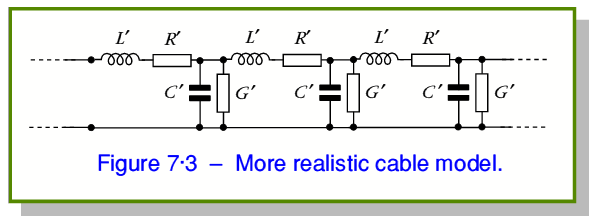
As a consequence of the above effects a better model of a cable is a series of elements of the form shown in figure 7·3.
Here the dissipative loss due to conductor resistance is indicated by a resistance-per-length value of  and loss due to the dielectric is represented by a conductance-per-length value of
  . As before, here I have used primes to emphasise that the values are per unit length and avoid confusion with total values or those of specific components.
The presence of the losses alters the propagation behaviour of the cables. The characteristic impedance and signal velocity now become
where  is the (angular) signal frequency and
  means the imaginary part. Note that, unlike the case for a ‘perfect’ cable, the impedance and velocity will now usually be frequency dependent. The frequency dependent cable velocity may be particularly significant when we are transmitting broadband signals as the frequency components get ‘out of step’ and will arrive a differing times. This behaviour is called Dispersion and is usually unwanted as it distorts the signal patterns as they propagate along the cables. Alas, all real cables will have some resistance/conductance so this effect will usually tend to arise. However, the good news is that if we can arrange that
then the two forms of loss have balancing effects upon the velocity and the dispersion vanishes. Such a cable is said to be ‘distortionless’ and the above requirement which has to be satisfied for this to be true is called Heaviside’s Condition, named after the first person to point it out.
The rate of energy or power loss as a signal propagates down a real cable is in the form of an exponential. For a given input power,  , the power that arrives at the end of a cable of length,
  , will be
where  is defined to be the Attenuation Coefficient whose value is given by
where  indicates the real part. For frequency independent cable values the above indicates that the value of
  tends to rise with frequency. This behaviour, plus some dispersion, are usual for most real cables. The question in practice is, “How big are these effects, and do they matter for a particular application?” Not, “Do these effects occur?”