In the previous article I introduced the use of the Fast Fourier Transform (FFT) and provided an application that employed this to produce power-frequency spectra for a section of a stereo sound file. This ability to quickly produce spectra is a very useful, however a single FFT doesn’t always get us the results we’d like. So I’d now like to introduce a new application, TrackFFTScan, and show how it can use used.
TrackFFTScan is similar to TrackFFT, but carries out a series of transforms. Detailed instructions for its use are in its !Help file. In practice you run it just like TrackFFT and the only obvious differences are that:
- It asks if you require ‘Apodisation’.
- As well as asking for a ‘start time’ it then asks for a ‘stop time’.
I’ll say more about apodisation later on. Initially I will give results where no apodisation has been applied.
The ‘stop time’ is needed because the application does a series of FFTs covering the portion of the sound file between these two times. Each individual FFT cover a run of 8192 pairs of left/right sound data samples, i.e. a chunk of duration 8192/44100 = 0·185 sec. Once you have given the application start and stop times it works out how many such chunks will fit into that part of the sound file, and proceeds to deal with them in sequence. As it does this it performs a power average over all the spectra it computes. It then saves the resulting averaged spectra for the left and right channels. To see why this is useful lets look at some real-world examples.
Let’s start with the use of broadband noise as a test signal. A common method for assessing the frequency response of an item is to provide it with noise as an input, and then FFT the output to reveal the spectrum.
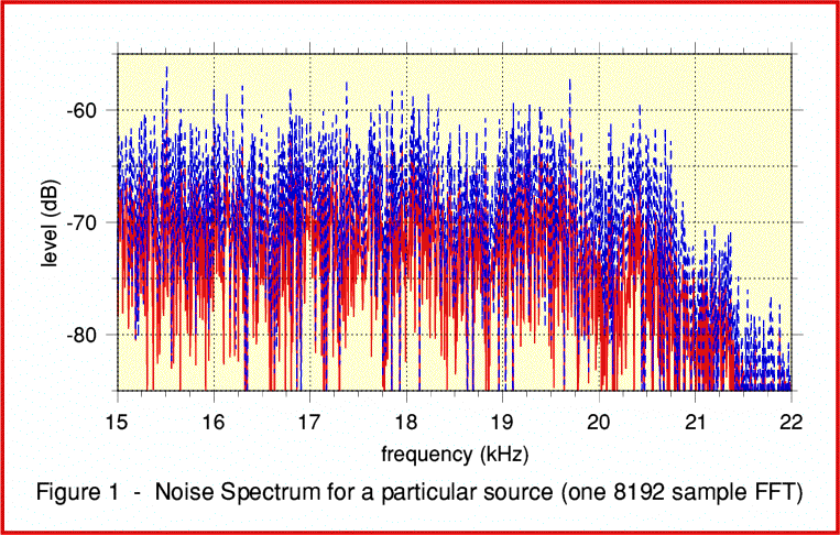
Figure 1 shows the result of doing this and obtaining spectra using TrackFFT. Two lines are plotted for the left and right channel signals. However you can immediately see that we have a problem interpreting the results! One of the consequences of using random noise is that the actual power level at each individual frequency of the spectrum varies unpredictably from one frequency to another. The average or typical level is determined – we can see it is around about the -70dB level in this example. But the random nature of the signal tends to hide any small features of the system response in a forest of spikes as the level jumps up and down unpredictably from one frequency to another.
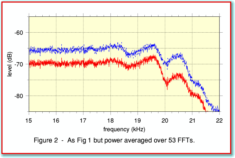
Figure 2 takes the same sound file as its source but used TrackFFTScan to obtain the spectra.
With TrackFFT I just did one transform that started 10 seconds from the beginning of the sound file. For Figure 2, I asked TrackFFTScan to do FFTs covering the period from 10 seconds to 20 seconds from the beginning of the file. It then did 53 FFTs and the spectra shown are the averaged results. You can see that this is much clearer than Figure 1. We can immediately see some apparent patterns in the response and how it falls away as we approach 22 kHz. We can also now clearly see that the two channels have different overall levels.
The improvement is because the fluctuations at each individual frequency vary randomly from one FFT chunk to the next. Hence when we combine the results taken from different parts of the sound data the random variations tend average away. This then reveals details which were otherwise lost. We now see a clearer representation of the average level at each frequency. This behaviour does, of course, depend on the random noise having the same statistical properties throughout the duration over which we did the scan and average.
However that isn’t all we can do with TrackFFTScan...
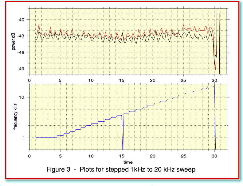
The second example I can show is based on a very different test signal. In this case it is a ‘stepped sweep’ signal. As with random noise this is another way of investigating the frequency response of a system. When you run TrackFFTScan it produces two output files on your ramdisc. One is the averaged spectra. The other is a report where each line provides a set of values derived from each successive FFT. These are the time of the relevant FFT, the frequency (in kHz) in that spectrum which had the highest power, and some power and distortion levels. (Full details are in the !Help file so I won’t explain them all here.)
Figure 3 illustrates an example of the use of the values from such a report file.
Here I have plotted the frequency on the lower graph, and the reported mean powers for the left and right channels on the upper graph. You can see that the results provide another way to determine the frequency response. (In this example the power level wobbles up and down. Knowing that the sound was recorded from a Test LP you may be able to deduce the reason for this regular wobble in level from studying the above plots!)
More generally, you can use TrackFFTScan to scan though a section of a test recording to identify the levels and frequencies involved. Then use it (or other Track applications) to examine sections in detail.
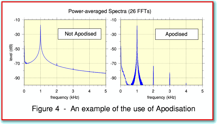
Now lets look at the effect of choosing apodisation. To illustrate this, look at Figure 4.
The example shown in Figure 4 is based on a recording of a 1kHz test sinusoid being played from a test LP. TrackFFTScan was used to produce a power spectrum averaged over 26 FFTs (5 seconds). You can see that without apodisation the 1 kHz tone generates large ‘wings’ that spread over a wide range of frequencies. This is an effect I referred to in an earlier article in this series when I introduced the TrackTHD application. However by apodising the data we produce a dramatic effect and the wings are reduced. This revels clearly the harmonics at 2, 3, 4, etc, kHz produced by distortion. Without apodisation these are only just faintly noticeable as slight ‘notches’ in the wings of the 1 kHz. But with apodisation their real level and detail is clear.
The use of apodisation and its effects are quite complex. So it doesn’t always produce an improvement in the results. For that reason I have provided it as a user option you can select when running TrackFFTScan. For purposes like looking for distortion it can be very useful, but check and compare the effects it has when using it for any given purpose. TrackFFTScan also lists the values it gets for distortion, in percentage terms, in its report file. This obviously may not mean anything if the input signal wasn’t a sinusoid. However – as you might expect from Figure 4 – distortion levels reported when you don’t use apodisation may be over-estimates as they can be inflated by the presence of the wings of the test tone! Used with care, TrackFFTScan with apodisation will give results for distortion far more quickly than the use of TrackTHD. But you might find it useful to check with TrackTHD as that may be more accurate.
Jim Lesurf
1200 words
19th Jan 2008
