Resampling Revisited
In the previous article on sound I looked at what happens if we try to use interpolation methods to resample a series of samples to obtain a new series at a different sampling rate. The results showed that interpolation methods can work reasonably well for signals which only have frequencies well below the sampling rate. But if the signal contains high frequencies the results can become quite seriously distorted. I only looked at linear and quadratic interpolations, and this showed that quadratic fits gave a better result. As you might expect, if we use higher orders of polynomials, or some other forms of function we can get even better results. But the complexity of the calculations rises, meaning the process takes longer. There is also a fundamental reason why this general approach can’t ever remove the distortions and errors which occur when the signal patterns include high frequency components.
In this article I want to outline a different approach that is formally based in Information Theory and which – in principle at least – can overcome the problems that lead to distortion. To do this, lets start with an example.
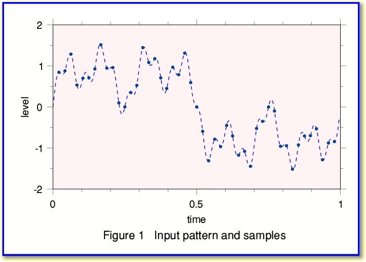
Figure 1 above shows a signal pattern (broken line) and a series of samples that represent this pattern. Although I won’t prove it here, one of the axioms of Information Theory is that the series of sample values can capture all of the information about the pattern provided we take the samples in accord with what Information Engineers know as the Sampling Theorem. This basically says that if all the frequency components in the pattern are less than a maximum,  , then we can make a ‘complete record’ of the information by ensuring that successive samples are no more than
  apart. The mathematics of Information Theory can be used to formally prove the above is correct. The converse is that we must sample at a rate
  to capture all the information in the pattern without problems.
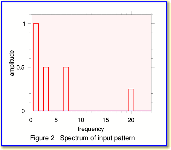
Lets now use the sample values shown in Figure 1 to compute the spectrum of our pattern. We can use Fourier Transformation for this. Again, I won’t bother will explaining all the details here, but the results in our example case come out as shown in Figure 2, below.
In this case I created the input signal using just four sinewave components, and the spectrum computed from the series of sample values shows this. (The frequencies here are all in terms of the number of cycles during the entire period of time for which we have samples.) Note that the spectrum was computed by a process that just used the sample values. The calculation which produced the above spectrum didn’t ‘know’ how I’d worked out the samples in the first place.
Once we know how much of which frequencies are present we find we are in the interesting position of being able to calculate the signal level at any instant during the period of time covered by our series of sample. i.e. we aren’t limited to just those instants where we originally had sample values! This means we can now use the spectrum information to work out what sample values we would have obtained at some other series of instants during the time the pattern was recorded. So we can use the spectrum to work out a new sample series. For example, we can take a series of samples made at 48 ksamples/sec, work out the spectrum, and then use this to calculate the samples we would have got if we’d sampled at 44·1 ksamples/sec.
The remarkable result, which can be proved by Information Theory, is that if we do this correctly the results are not ‘interpolations’. They are genuinely the values we would have obtained if we’d sampled at 44·1 ksamples/sec in the first place. I have left out many of the details of the above argument. But formally speaking, the above can be shown to be rigorously correct according to the mathematics of Information Theory. It means that if we know how to apply the above we can resample the information without any distortion at all. However there is a price for this precision. The process is quite a complex and long calculation, so can take a lot longer than simple low-order interpolation. Fortunately, there turns out to be a ‘short cut’, but rather than reveal it here it will help later on if we investigate something else. This may seem like a diversion, but stay with me...
Let us now suppose that instead of resampling to a different sample rate, our interest is in filtering the signal to remove some of the frequencies that are present in the original pattern. There are various techniques for filtering the sound pattern. I used one approach a few articles back when I wrote an article on ‘DSP’ with an example that provided a notch (rejection) filter that can be used to suppress an unwanted tone from a recording. From what I’ve written above we can now see another method. Take the samples and Fourier Transform them to get the signal spectrum. Then change some of the values of the amplitudes and/or phases of the frequency components in the spectrum.
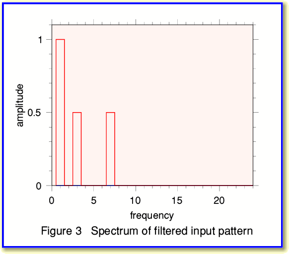
To illustrate this, take the spectrum of our initial signal pattern and set to zero the amplitudes of any frequency components above, say, 15 cycles. The result then looks like Figure 3. If we compare this with Figure 2 we can see that the component at 20 cycles has gone.
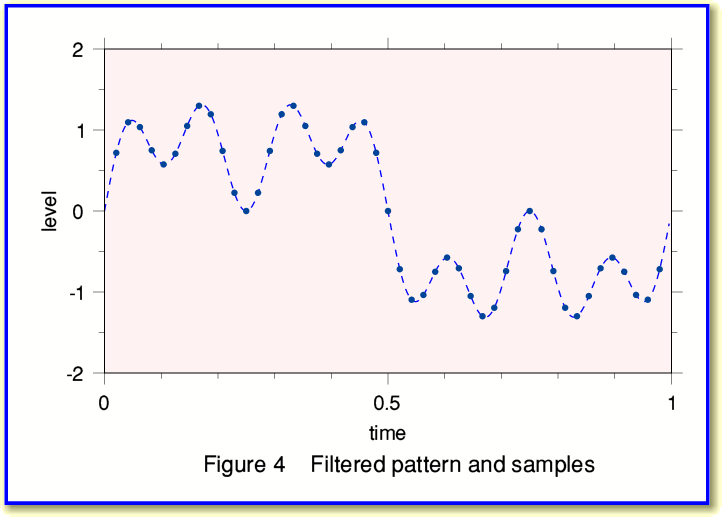
We can now use this filtered spectrum to work out what samples we would have obtained in the absence of the high frequency components. The result is shown in Figure 4 and we can compare this with Figure 1 to see the change produced by the filtering.
In the above example, Figure 4 shows the sample values at the same instants as for our original signal pattern. i.e I kept the sample rates of the input and output the same to make the effect of filtering clear. But we could have used the filtered spectrum to work out the sample values we would have got at other instants if we’d used a different sample rate...
Now there are various reasons why we might want to filter the signal pattern. For example, the components we wish to remove may be annoying for some reason. But when it comes to resampling data to a different rate there is a very important reason why we may have to filter the pattern. This stems from the Sampling Theorem as we discussed earlier. When sampling audio at 48 ksamples/sec the input sounds can have frequencies up to just under 24 kHz. i.e. the input had to be limited to less than 48/2 = 24 kHz. If we now want to resample the series of 48ks/sec data to produce an output at the CDA rate of 44·1 ks/sec we have to ensure that the result is indistinguishable from that we’d have got if we’d sampled at 44·1 ksamples/sec in the first place. But the Sampling Theorem would then have required us to ensure the input didn’t have any frequencies equal to or above 22·05 kHz for this data to be OK. Thus we may have a problem. If our 48 ks/sec data contains any signal components in the frequency range between 22·05 kHz and 24 kHz then our resampling process must remove these or the result will be distorted in some way.
As a result of the above, we can resample if we wish by using the following method:
- 1) Take the 48 ks/sec data and divide it into a convenient series of ‘chunks’ of successive values.
- 2) Fourier Transform each chunk to get the spectrum of the pattern.
- 3) Set to zero any amplitudes for frequencies in the range from 22·05 kHz up to 24 kHz.
- 4) Use the resulting, filtered, spectrum to work out the values at the instants we’d have sampled if we’d used 44·1 ks/sec.
- 5) String the chunks of 44·1 ks/sec samples back together.
Note that step (3) is vital when converting 48 ks/sec data into 44·1 ks/sec form. One problem with simple methods like quadratic interpolation is that it doesn’t do this, so is doomed to give problems whose severity depend on the details of the input pattern. Hence the tendency with simple interpolation for the distortion level to rise if we have high frequencies in the signal patterns to be processed.
There are some other requirements and details I’ve omitted to avoid making the topic even more complicated, but the above can work well. The snag is that we (or our computer!) has to do a lot of work to transform the information back and forth. The good news is that the above links in with the general topic of ‘filtering’ and points to other ways to get the same end-result. It turns out that there are ways to combine steps (2)-(4) of the above into one computational step. Thus making the process much easier. For that reason in DSP and IT the topics of resampling and filtering are often treated as being two facets of the same general process, and can be tackled by various methods.
1550 Words
Jim Lesurf
11th Sep 2007

