Resampling - Part 1
In the previous article I showed how timing problems mean that Iyonix sound recordings made at any rate other than 48 ksamples/sec are distorted by a hardware problem. As a result, if you use !AudioIn with your Iyonix to make recordings at the standard CD rate of 44·1 ksamples/sec the sound quality will be seriously degraded. Recordings at 48 ksamples/sec don’t have this problem. But the snag is that they aren’t suitable for an Audio CD!
Recording engineers regularly encounter the need to take a recording made at one sampling rate and generate an output with a different sample rate. This process is known as “resampling” and it involves computing a ‘new’ series of sample values from the data. Professionals will tend to use systems which do this process by numerical techniques that are based on Information Theory and can be formally shown to give the correct results. i.e. They produce a series of samples which genuinely have the values we would have obtained if the recording had originally been made at the new rate. So in principle dealing with the above problem is easy. First we use the Iyonix to make a 48 ksamples/sec recording. Then we use one of these resampling methods to compute the series of samples we would have got if we’d used 44·1 ksamples/sec and that had worked perfectly. Once that has been done, the results can be written onto an Audio CD with no distortion problems. Easy!
Alas, there is a snag. The formally correct methods tend to be quite demanding in terms of computation, and hence will be quite laboriously slow on an Iyonix or other RO machine. Our Achilles Heel here is the absence of a Floating Point Unit in the processors we use. So are there any swifter alternatives?...
Some existing applications use an approach based upon linear interpolation. This works by putting each ‘new’ resampled value on a straight line joining the two samples in the original data that are closest to it in time.
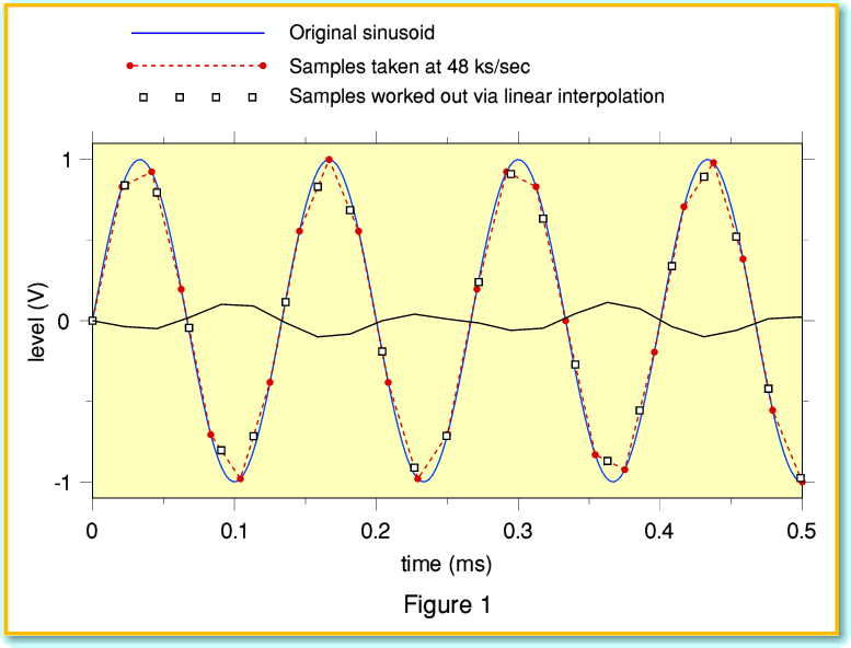
Figure 1 illustrates how this works, and the kind of results it produces. The initial signal for this example is a 7·5 kHz sinusoid (solid blue line). The round (red) blobs represent a series of samples of this sinusoid taken at 48 ks/sec rate. The broken (red) line essentially “joins up the dots” of this series of 48 ks/sec values. The open squares show the values on these lines at a series of instants that are 1/44100 th of a second apart. Hence these open squares indicate the values we get if we use linear interpolation to work out a series of samples at the CD rate from the 48 ks/sec data. You can see that in general, these results don’t sit neatly on the input sinusoid! The solid black line of relatively low amplitude shows the pattern of difference between these interpolated samples and the ones we would have got if we’d sampled the input sinusoid at 44·1 ks/sec in the first place. For the 7·5kHz sinusoid the amplitude of this error pattern is equivalent to an average distortion level of around 8%.
The error and distortion arises because the actual waveshape is curved, not a series of straight lines between the original samples. From this we can expect that the higher the signal frequency, the greater the curvature, and so the worst the distortion or errors will be.
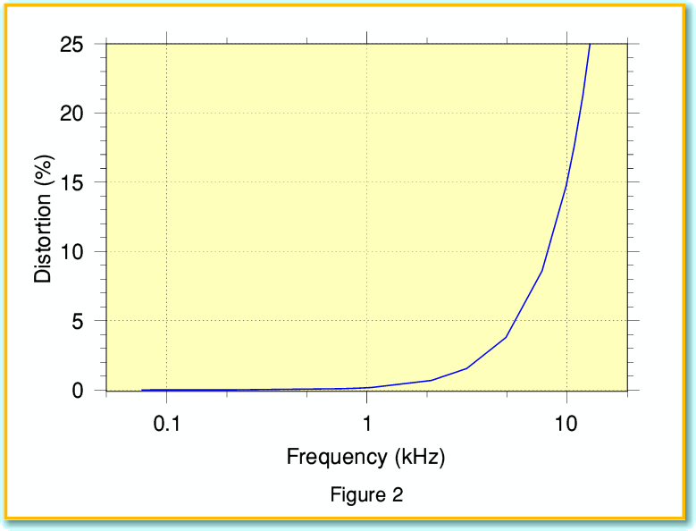
Figure 2 indicates how the distortion level produced by linear interpolation rises with the frequency of an input sinusoid. It can be seen that for frequencies below one or two kHz the distortion level is reasonably low, but by the time we reach 5 kHz or more the distortion is rising rapidly. By 10 kHz it is over 15%, and by 15 kHz it reaches over 30%! Note that the distortions generated are not ‘harmonic’ as they depend on the relative ’phases’ of 48 kHz, 44·1 kHz and the signal frequency. The results can be quite nasty unless the original input has virtually no frequency components above a few kHz. It is also worth noting that – unlike many physical causes of distortion – the level of distortion is essentially unaffected by the signal amplitude. This means that quiet sounds will be distorted to the same degree as loud sounds. Not a happy result.
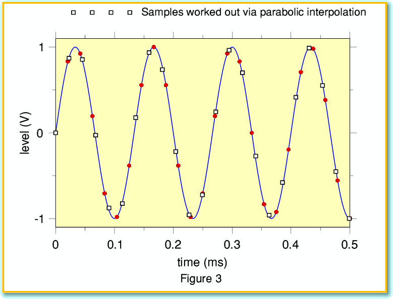
So can we do any better?... yes, we can. Figure 3 illustrates the results of doing parabolic interpolations, again for a 7·5 kHz sinusoid as our test waveform. As with Figure 1 the solid (red) blobs are the original samples, and the solid (blue) line is the sinusoid represented by those samples. The open squares show the resampled values at CD sampling rate when calculated using parabolic interpolation. If we compare this with Figure 1 we can see that the resampled values computed are much closer to being on the original waveform. This immediately indicates that we can expect the level of distortion to be much less than when we used linear interpolations.
The drawback of this method is that it requires a more complicated calculation. For example resample value calculation linear interpolation uses just the two original samples closest in time to each new value we wish to estimate. And we only have to solve for a linear expression. The parabolic interpolation requires the three closest values in time, and we have to solve and use a quadratic for each resampled value. However the results are distinctly better as we are now taking into account to some extent the curvature of the waveform.
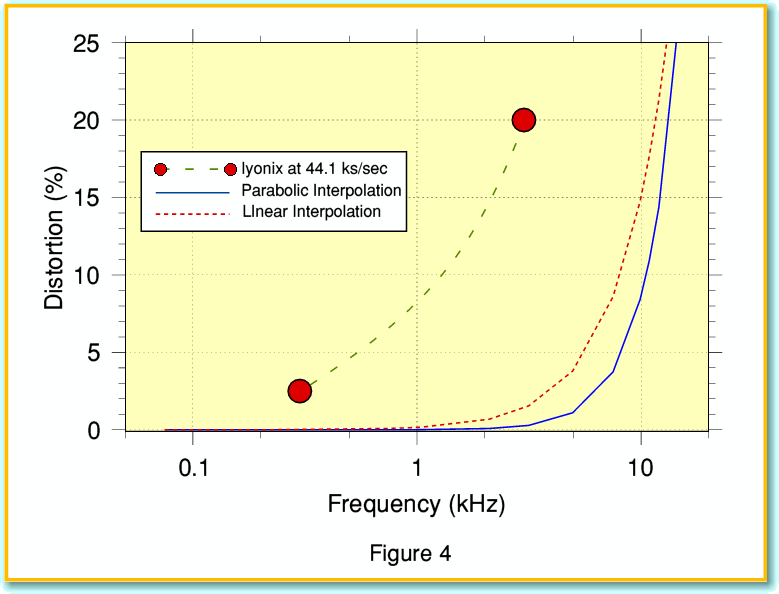
The continuous line in Figure 4 shows how the distortion level varies with frequency for a parabolic fit. The broken (red) line shows the results for a linear fit. It can be seen that for signal frequencies much above 5 kHz the improvement probably isn’t worthwhile as we still get high levels of distortion. However for lower frequencies the improvement is quite significant.
| Frequency (kHz)
|
0.75
|
1.0
|
3.0
|
5.0
|
10.0
|
| Linear Distortion (%)
|
0·08
|
0·17
|
1·54
|
3·79
|
17·67
|
| Parabolic Distortion (%)
|
<0·01
|
0·01
|
0·28
|
1·10
|
10·92
|
The table lists some example values. In neither case is the result exactly ‘hifi’. Even by the standards of the 1960’s a distortion level of around 0·1% or less would be regarded as desirable. With some simple low-harmonic forms of distortion up to 0·5% might be acceptable, but values well above 1% would generally be regarded as too high for comfort. That said, the parabolic approach does do better than linear interpolation, and for inputs that are largely composed of frequencies below about 5 kHz may sound acceptable.
At this point it is worth reminding ourselves of the results in a previous article which considered what happens if you use an Iyonix to make recordings at the CD sampling rate of 44·1 ks/sec. Due to the timing problems I discussed, the results then would have a distortion level of around 20% at 3 kHz and 2·5% at 300 Hz. These values are vastly higher than we would get by taking samples at 48 ks/sec and then using parabolic interpolation to generate CD samples. So although the interpolation method is far from perfect, it is much better than simply using the Iyonix to sample at CD rate. By using parabolic interpolation we can reduce the distortion level by a factor of around a hundred!
In practice, although enthusiasts often expect an audio system to have a frequency response extending up to around 20 kHz, the actual music often has little energy at frequencies well above 5 kHz. Also, one of the main uses people have in mind for a sound sampling input is to make digital recordings of old LPs and Cassettes which they then put onto CD-R’s. The idea being both to preserve treasured recordings, and make them easier to play. In reality, many such original sources will already have high levels of distortion at high frequencies, as well as limited amounts of high frequency content. This means that in reality the concern can be with ensuring that the recording/resampling methods don’t add more distortion than was already present with such material. Not perfect, but fit for the task in hand.
In the next article I will continue to investigate resampling, and – I hope – provide an example application that Iyonix owners can use to get better results.
Jim Lesurf
1500 Words
24th Jul 2007