Pump up the Volume!
In this article I want to examine being able to change the volume level (amplitude) of the sounds represented by a sound data file. As in the previous articles in this series I am assuming the sound files are of the ‘data’ type saved and used by !CDBurn or !CDVDBurn. As before, I have given Paul a program as a useful working example, and I will use that to illustrate the points I wish to make.
The new program is called !TrackGain. To use it, first set it up in a similar way to the previous example programs. It has an internal Path file and you should ensure this contains the full path name of the directory for input and output. In this case it expects to find two directories, CDtrack_in and CDtrack_out, inside the directory pointed to by the content of Path. Create these directories, and put the data file you want to use as input into the CDtrack_in directory. Then run !TrackGain in the usual way.
This opens a taskwindow and asks for the name of the input file. One you have given this it asks what change in level (gain) you require. The program expects a value in decibels. (dB). This means that a value of “0·0’ will leave the level unchanged. A value of ‘10·0’ means the resulting output will be ten times as powerful when listened to, and a value of ‘-20·0’ means it will be a hundred times quieter. i.e. positive values make the result louder, and negative ones quieter.
Figure 1
Values in dB are – by definition – a power or energy ratio. But dB values can be used in two ways. One way is to say that “we have changed the level by XdB”. This tells us how much the power (volume) level has been altered by something. This is the meaning used for the values you give to !TrackGain. A different way is to say that “this signal power is YdB compared to some reference level”. In this article you’ll see values like this referred to as ‘dBFS’. This means a signal (sound) power lever relative to the ‘Full Scale’ level for audio CD. So ‘-10dBFS’ means ‘a sound power that is 10dB below the largest possible level that CD data can represent’.
Once you’ve given it a gain value the program asks if you want ‘dithering’. I’ll explain this in a later article. For now, just choose ’y’ or ’n’, then press return. (In fact, the program simply looks at the first character of what you type at this point and if it is either a ‘y’ or a ‘Y’ employs dithering. Anything else, and it does not employ dithering. So you can type ‘yes’ and press return if you want dithering or type ‘elephants’ and press return if you don’t!)
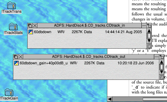
The program then works its way though the input file, reads the values, scales them by the specified gain, and writes the results into a new file in the CDtrack_out directory. Note that the new file has a name which starts like that of the source file, but has the chosen gain value appended to it, and at the end either says ‘_u’ or ‘_d’ to indicate if it was ‘undithered’ or ‘dithered’. (This assumes your filing system can cope with the long files names!) Figure 1 shows example input and output file in their filer windows.
Figure 2 shows the spectra for an input file containing a 1 kHz sinewave at the -60dBFS level (broken black line) and for a file produced from this using !TrackGain to apply a gain of +50dB (continuous blue line).
In practice, the most obvious use for !TrackGain would be to boost the recorded volume level if you have a recording that is inconveniently quiet. To assess this, you could first use !TrackStats to determine the sound levels recorded in a file, then use !TrackGain to change these as seems appropriate. When doing this, we have to be aware of a few traps, though...
The most obvious potential problem is that you may increase the signal levels by too much. This can lead to a serious problem called clipping. To guard against this, !TrackGain monitors the output it is producing and issues a warning if it occurs. The problem arises because CD audio data is stored as a series of 16-bit integers. One bit is used for the ‘sign’ of the value and only 15 bits are available for the magnitudes. This means we can only represent values as a series of integers over the range from -32767 to +32767. Hence if we calculate any gain-changed values which are outside this range we find that the CD audio data format has no way to represent them, and the result won’t play correctly. To avoid this, !TrackGain checks the changed values to see if any are too large. Any which are ‘out of range’ are limited to the maximum possible values, and the program prints out a warning for the user. If this occurs you should note that the sound in the output will be distorted and information has not been correctly transferred to the output file. In general, if you encounter such a warning you should re-run the program and apply a lower gain to avoid the problem.
Since this is ‘Archive’ you are probably familiar with binary integers, and perhaps found the values I gave for the limits puzzling. This is because 215 = 32768 not 32767. Why is the limit ‘off’ by one? The reason is the way the CD audio system uses integer values to represent the actual sound information, and is illustrated in Figure 3.
 Figure 3
This shows two plots. The broken (black) line shows what we get if we look at ‘real’ values and plot them against the values we obtain when we simply convert them into an integer.
Looking at the broken line we can see that all values from -0·999... to +0·999... produce an integer value of ‘0’. This means that the broken line looks like a ‘staircase’, but with the tread around ‘0’ being double the width of all the others.
We need to represent a smoothly variable (real) quantity – the air pressure variations caused by sound waves – in terms of a series of integer values. This means we have to quantise. the values, and we want all the steps to be of the same size. Hence the quantisation has to produce uniform ‘steps’ on the staircase.
If you look at the source code for !TrackGain you will see I have written a specific procedure for the required conversion. The results are illustrated by the continuous (blue) line in Figure 3, and you can see the steps are now uniform. However this quantisation method means the total range we can cover has been slightly reduced since we have lost the ‘double-width’ step around zero. Thus for safety we have to limit the range to ±32767, not ±32768.
In principle, even this limit isn’t absolutely ‘safe’. A full explanation of the reason is quite complex, and involves a fair amount of understanding of Information Theory. However I can give an example to illustrate the problem.
Consider an ‘impulse’ – i.e. a ‘click’. This may contain energy over a wide range of frequencies. However CD recordings have to be filtered when being recorded, and only frequencies up 22kHz will appear on the recording. From a theoretical point of view, it can be argued that ‘ideal’ filters for recording (and replay) do not alter the relative amplitudes or phases of any frequency components up to 22kHz, but suppress entirely any frequency components at higher frequencies. This leads to results of the type indicated in Figure 4. Here the continuous (red) line represents the ‘click’ before it was filtered. The broken (blue) line represents the filtered waveform which we then sample. The squares represent the sampled values.
If we look at the sample values recorded using this process we can see that our idealised filter leads to the click producing just one non-zero sample value. The removal of the frequencies above 22kHz actually produced a pattern called a sinc waveform. Note that for the example shown in Figure 4 I assumed that the click occurred precisely at one of the sampled instants. The result is a pattern of sample values which are identical to if we’d just detected one instant when the sound had a non-zero level. When we use the sample values to reconstruct an audio waveform we will get an output waveform having the sinc pattern (broken line). This only differs from the original click in that the components above 22kHz have been removed. Hence if we can’t hear such high frequencies, the result should sound indistinguishable from the original click.
The above summarises the standard view which is presented in many textbooks on sampling and conversion between analog and digital representations of waveforms/information/patterns. However there is an important detail which most textbooks then ignore. This is illustrated in Figure 5. Here the click and filters are the same as before, but the instant when the click occurred is mid-way between two of the sampled instants.
If we compare Figures 4 and 5 we can see two distinctions. Firstly. that when the click didn’t occur exactly at a sampled moment, the sample values around this instant won’t all be zero. We no longer have an isolated non-zero value to represent the filtered click. The second difference is much more important. If we look back at Figure 4 we can see that the non-zero sample value is at the peak of the waveform which will be reconstructed when the data is used to replay the sounds. However in Figure 5 the largest sample values are on the ‘shoulders’ of the waveform peak, so don’t show the maximum amplitude which the replay system will have to produce when the sample are used to reconstruct a waveform. In both cases, however, the desired output waveform has the same shape and overall amplitude. It just occurs at a slightly different time.
The problem is as follows: We may scan though the sound data with a program like !TrackStats and find that the peak values of the sound sample were less than the maximum possible individual values possible for CD data. We might then use !TrackGain to scale up the values so that the largest samples are just at the maximum permitted level of ±32767. However – if the data contained any information similar to that used in Figure 5 – the player will then have to produce levels which were greater than the peak permitted/expected level!
For most realistic music and speech, this problem is very unlikely to arise. However if we wish to avoid running into problems we have to be cautious when changing the volume of the sounds. This means ensuring there is a decent safety margin and none of the samples come too close to ±32767. Taking the above example as a guide, this would mean ensuring that none of the sound samples exceed the -4dBFS level. Hence I’d recommend ensuring this when using a program like !TrackGain. To take an example, lets assume we start with a sound file where !TrackStats shows that the highest peak level is, say, -18dBFS, and we want to boost the volume as much as may be ‘safe’. We can use !TrackGain to apply a gain of +14dB (i.e. 4 less than 18). If we check the result with !TrackStats we should find that the highest peak level isn’t more than -4dBFS – low enough to avoid any problem.
29th Jun 2006
Jim Lesurf