YouTube Audio Quality - How Good Does it Get?
You Tube is clearly used by a very large number of people. In general, they will be interested in watching videos of various types of content. One specific purpose is that it gets used to distribute, and make people aware of, audio recordings. A conversation on the “Pink Fish” webforum devoted to music and audio set me wondering about the technical quality of the audio that is on offer from You Tube (YT) videos. The specific comment which drew my attention was a claim that the ‘opus’ audio codec gives better results than the ’aac / mp4’ alternative. So I decided to investigate...
Ideally to assess this requires a copy of what was uploaded to YT as a ‘source’ version which can then be compared with what YT then make available as output. By coincidence I had also quite recently joined the Ralph Vaughan-Williams Society (RVWSoc). They have been putting videos up onto YT which provide excerpts of the recordings they sell on Audio CDs. These proved excellent ‘tasters’ for anyone who wants to know what they are recording and releasing. And when I asked, they kindly provided me with some examples to help me investigate this issue of YT audio quality and codec choice.
For the sake of simplicity I’ll ignore the video aspect of this entirely and only discuss the audio side. The RVWSoc kindly let me have ‘source uploaded’ copies of two examples. The choice of audio formats that YT offered for these videos are as follows:
|
Pan’s Anniversary Available audio formats for HZHVTr1w6L8: ID EXT | ACODEC ABR ASR MORE INFO ------------------------------------------------------------ 139-dash m4a | mp4a.40.5 49k 22050Hz DASH audio, m4a_dash 140-dash m4a | mp4a.40.2 130k 44100Hz DASH audio, m4a_dash 251-dash webm | opus 153k 48000Hz DASH audio, webm_dash 139 m4a | mp4a.40.5 48k 22050Hz low, m4a_dash 140 m4a | mp4a.40.2 129k 44100Hz medium, m4a_dash 251 webm | opus 135k 48000Hz medium, webm_dash VW on Brass Available audio formats for KsILRbZtTwc: ID EXT | ACODEC ABR ASR MORE INFO ------------------------------------------------------------ 139-dash m4a | mp4a.40.5 50k 22050Hz DASH audio, m4a_dash 140-dash m4a | mp4a.40.2 130k 44100Hz DASH audio, m4a_dash 251-dash webm | opus 149k 48000Hz DASH audio, webm_dash 139 m4a | mp4a.40.5 48k 22050Hz low, m4a_dash 140 m4a | mp4a.40.2 129k 44100Hz medium, m4a_dash 251 webm | opus 136k 48000Hz medium, webm_dash |
The ‘ID’ numbers refer to the audio streams. Other ID values would produce a video of a user-chosen resolution, etc., normally accompanied by one of the above types of audio stream.
One aspect of this stands out immediately. This is the variety of audio sample rate (ASR) options on offer. However in each case only one version of a RVWSoc video was uploaded, at a sample rate chosen by the RVWSoc. I had expected to see a choice of YT output audio codecs (compression systems), but was quite surprised, in particular, to see ASRs as low as 22·05k on offer as that means the YT audio would then have a frequency range that only extends to about 10kHz!
Given the main interest here is in determining what choice may deliver highest YT output audio quality I decided that analysis should focus on the higher, more conventional rates – 48k and 44k1. In addition, the above shows that – since in each case only one source file (and hence only one sample rate) was uploaded – some of the above YT output versions at 48k or 44k1 have also been thorough a sample rate conversion in addition to a codec conversion. That introduces another factor that may degrade sound quality! In this case I had copies of what had been uploaded, so could determine which of the YT output versions had been though such a rate conversion. For the present examination, I will therefore limit investigation to the YT output that maintains the same ASR as the source that was uploaded, so as to dodge this added conversion. Unfortunately, in general YT users probably won’t know which output version may have dodged this particular potential bullet! Choosing the least-tampered-with output therefore may be a challenge in practice for YT users.
Pan’s Anniversary [48k ASR 194 kb/s aac(LC) source audio]
I’ll begin the detailed comparisons with the video of an excerpt from the CD titled,“Pan’s Anniversary”. The version uploaded contains the audio in the form encoded in the aac(LC) codec at a bitrate of 194 kb/s and using a sample rate of 48k. The audio lasts 4 mins 54·88 sec. The table below compares this with the same aspects of the high ABR versions offered by YT.
| version | codec | ABR | bitrate (kb/s) | duration (m:s) |
| source | aac(LC) | 48k | 194 | 4:54·88 |
| YT-140 | aac(LC) | 44k1 | 127 fltp | 4:54·94 |
| YT-251 | opus | 48k | 135 fltp | 4:54·90 |
We can see that YT-140 uses the same codec as the source, but alters the information bitrate, and the ASR. YT-251 transcodes the input aac(LC) into the opus codec, but doesn’t alter the sample rate. Both of the YT versions are of longer duration than the source uploaded. By loading the files into Audacity and examining the waveforms by eye it became clear that the YT versions were not time-aligned with each other, or with the source.
To avoid any changes caused by alteration of the ABR I decided to concentrate on comparing the source version with YT-251 – i.e. where the output uses the opus codec, not aac, but maintain’s the source sample rate. Having chosen matching sample rates the simplest and easiest was to check how similar two versions are is to time-align them and then subtract, sample by sample, each sample in a sequence in one version from the nominally ‘same instant’ matching one in the other. If the patterns are the same, the result is a series of zero-valued samples. If they don’t match we get a ‘difference’ pattern. However, before we can do this we have to determine the correct time-offset to align the sample sequences of the two versions.
In some cases that can be fairly obvious from looking at the sample patterns using a program like Audacity. But in other cases this is hard to see with enough clarity to determine with complete precision. Fortunately, we can use a mathematical method known as cross-correlation to show us the time alignment of similar waveform patterns. (See https://en.wikipedia.org/wiki/Cross-correlation if you want to know more about cross correlation.) This also can show us where the best alignment may occur in terms of any offset between the two patterns of samples being cross correlated.
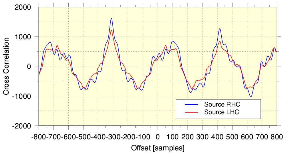
The above graph shows the result of cross correlating a section of the source and YT-251 versions of the audio. (The red and blue lines show the Left and Right channels of the stereo.) The results cover offsets over a range of +/- 800 samples. The process used 180,000 successive sample pairs from each set of samples. i.e. about 3·75 sec of audio from each. The best alignment is indicated by the location of the largest peak. If the sample sequences were already aligned this would happen at an offset = 0. However here we can see that the YT-251 version is ‘late’ by just over 300 samples.
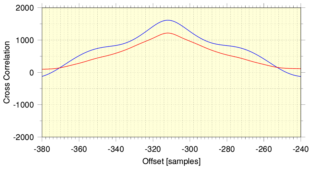
Zooming in, we can see that the peak is at an offset of -312 samples. Which at 48k sample rate corresponds to YT-251 being 6·5 milliseconds late. Having determined this I could trim 312 samples from the start of each channel of YT-251 and this aligned the two series of samples. (I also then had to trim the end to make them of equal length.) Once this was done it becomes possible to run though the samples and take a sample-by-sample difference between the source version and YT-251. This different set then details how the YT-251 output differs from the source version.
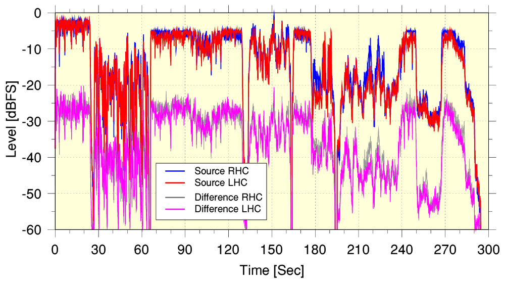
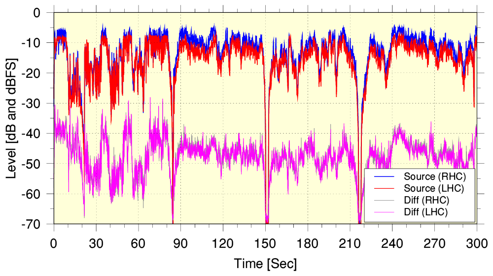
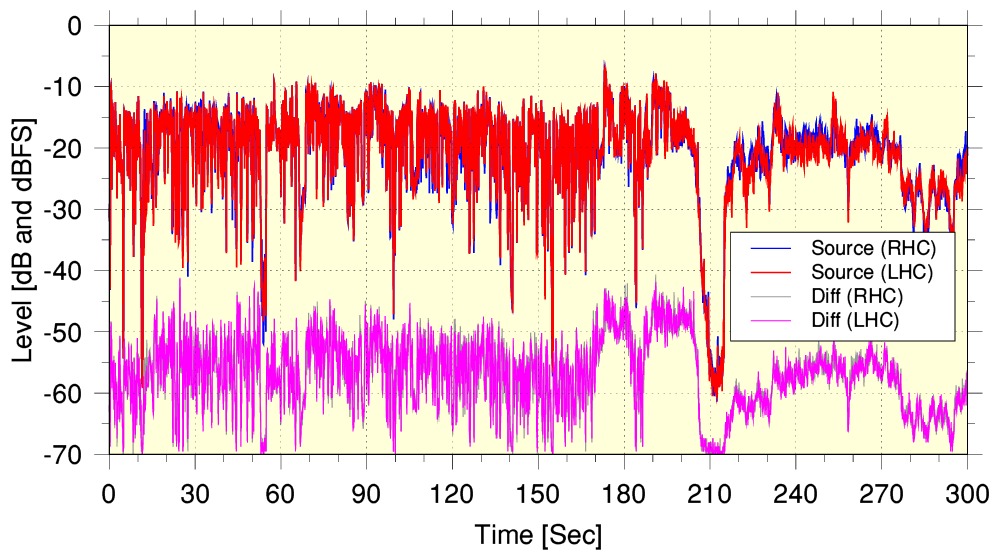
The graph above shows how the rms audio power level of the audio varies with time. The red and blue lines show the levels in the Pan’s Anniversary source file. The grey and purple lines show the power levels versus time obtained from subtracting the source file sample values from the audio samples from YT-251. Ideally, we’d wish to find a subtraction like this producing a series of zeros as the difference samples. This is because such a result would tell us that the output was identical to the input and going via YT had not changed the audio at all! However in practice the above results show this clearly is not the case! There is a residual ‘error’ which is typically somewhere around 20dB below the input (and output) musical level.
In traditional terms for audio, 20dB would be regarded as a very poor signal/noise ratio. And if the change was considered as being equivalent to conventional distortion it would be assumed to indicate a level of around 10% distortion! So it represents a rather underwhelming result. However a more benign interpretation may be that it arises as a result of the process applied by YT slightly altering the overall amplitudes of the waveforms so they don’t quite match in size – hence leave a non-zero difference when the input and output are subtracted. With this in mind we can compare the input and output samples using other methods that aren’t sensitive to an overall change in signal pattern levels.
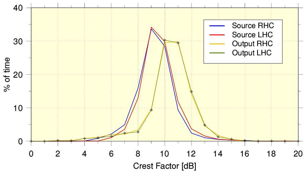
The above graph compares the input and output files in terms of Crest Factor. This measures the peak-rms power level difference of the waveform shapes defined by the series of samples. The red/blue lines show the Left and Right channel results for the source file sent to YT. The orange/green lines the equivalent results for YT-251. To obtain these results each set of samples was divided up into a series 0·1 Sec sections. The peak and rms power level of each was calculated, and the above shows how often a given value was obtained, grouped into 1dB wide statistical ‘bins’. For a pure sinewave the peak/rms crest factor is 3dB. i.e. the peak levels of a sinewave are 3dB larger than the rms power. For well recorded music from acoustic instruments the Crest Factor tends to be in the range from a few dB up to well over 10dB for the most ‘spiky’ waveforms.
The result is interesting as we can see that the YT-251 output clearly exhibits a different Crest Factor distribution to the source file. It seems doubtful this could be produced by a simple change in the overall signal pattern level. (e.g. a volume control does change the overall level, but it should not change the shape of the audio waveform, and hence should leave the Crest Factor unaltered. (If it did alter this, you’d be advised to replace the control with one that worked properly!) It is particularly curious that the Crest factor seems to be increased by having the audio pass though the YT processing. Although possibly this may arise due to an input which is aac(LC) coded being transcoded into ‘opus’ codec form. OTOH perhaps YT apply some form of ‘tarting up’ to make audio ‘sound better’...
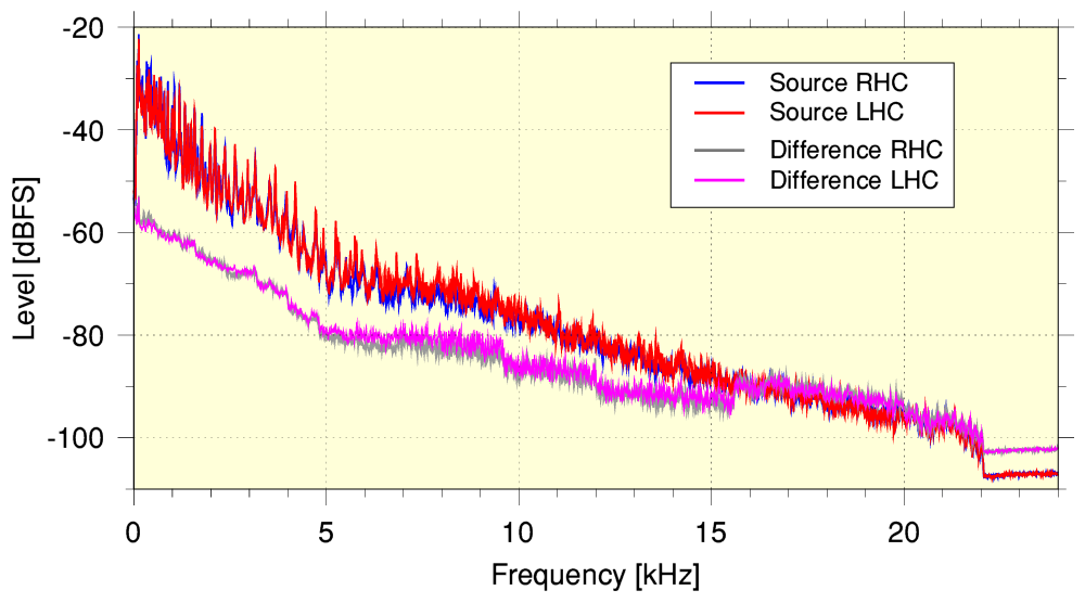
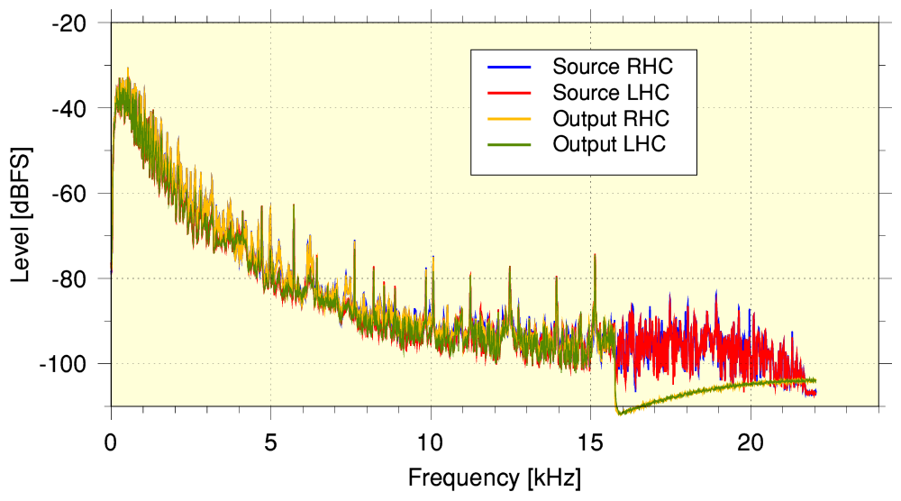
A more familiar way to show the character of an audio recording is to plot its spectrum. The above graph shows the spectrum of the Pan ‘source’ file and of the series of samples obtained by subtracting the YT-251 output sample series. We can then say that - at any given frequency - the bigger the gap between these plotted line, the closer the YT-251 output is to the source supplied to YT. Looking at the graph we can then see that the results indicate that the faithfulness of the YT-251 result to the input is at its best at low frequencies where the gap is widest and the contributions to the overall signal level are greatest. However at higher frequencies the level of the error becomes a larger fraction of the input. And above about 16kHz the error level quite similar to the input level. The implication being that the original details in the source above about have essentially been lost. They may have been replaced by something generated to ‘fake’ this lost information in a plausible manner.
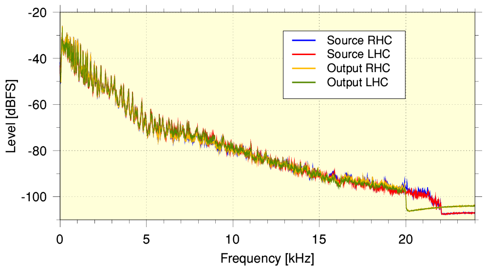
In fact, if we compare the spectra of the input with that of the output we can see that the YT-251 output using the opus codec has essentially removed anything from the source that was above 20 kHz. This is replaced by an HF ‘noise floor’ produced via a process like dithering, probably employed to suppress quantisation distortion, etc. We can also see that the source, although at a 48k sample rate, has a sharp cutoff at just over 22 kHz. This indicates that that although what was submitted to YT was at 48k sample rate it was actually generated from a 44k1 (i.e. audio CD rate) version. The behaviour of the above spectra may well be another sign of changes that also produced the change in the typical Crest Factor distribution.
Having applied the above analysis to an example that produced a YT output using the opus codec we can now examine another example which uses aac for the output to compare that with the use of opus.
Vaughan-Williams on Brass [44k1 ABR 127 kb/s aac(LC)]
In this case the choice of source file had an aac audio content at an ASR of 44k1. This was chosen to match the sample rate of YT-140 and thus avoid any sample rate resampling effects. As with the previous “Pan’s Anniversary” example the YT-140 output was of a different duration to the source file, and not sample-aligned. So as before, I edited the output samples to trim them to a sample-aligned series that matched the timing of the source version.
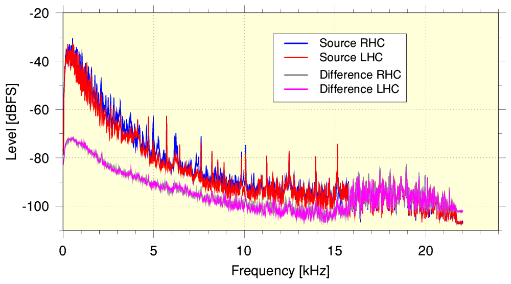
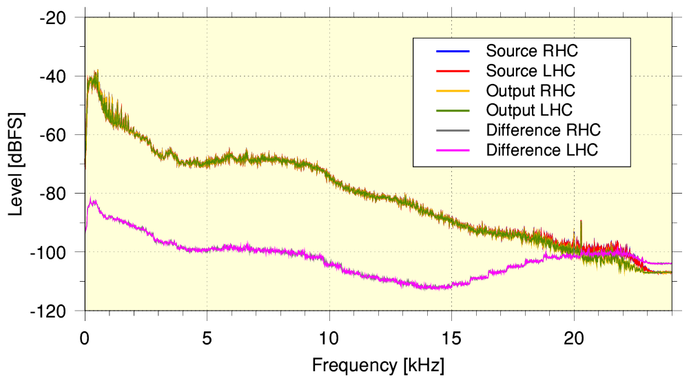
The graph above shows the time-averaged spectra of the source file and the difference between this and the YT-140 output. This represents the residual error level
As with the earlier YT-251 example, the above shows the source signal level versus time, and the level versus of time of the sample-by-sample difference between the source and the YT output (now YT-140) level. In this case the error level seems to be around -30 to -35dB compared with the source which is an improvement on the earlier YT-251 example. Viewed as distortion it would be equivalent to a level of around 3% or less.
More broadly speaking, the results look similar to the previous example. However...
...when we compare the actual spectra of the input and output we find that the output now has its high-frequency range cropped off at just under 16kHz! This is distinctly lower than the range present in the 44k1 sample rate aac input submitted to YT.
It is also worth noting that although the YT-251 example’s output spectrum seems to extend to around 20kHz we found that the part above about 15kHz looked like being ‘all error’! i.e. not the source HF details but some sort of facsimile!
Overall therefore, we might judge the YT-140 example to be, technically, more accurate than the YT-251 example. But to tell if this result was a general one we’d need to examine more examples. And given the changes in the applied high-frequency cut-off, we might also find that allowing the sample rate to altered might, overall, yield a different outcome! So the above results are interesting, but raise further questions which deserve future investigations.
BBC iPlayer as a comparison [48k ASR 320 kb/s aac]
In 2017 the BBC experimented with streaming BBC Radio 3 using flac in parallel with their standard iPlayer output formats. They did this for two reasons. One was to assess the practical requirements they would need to support if it became a standard. The other was to investigate if it produced audibly ‘better’ results. Some programmes were parallel streamed in days leading up to the Proms of that year. And almost all of the Proms were also streamed in flac format as well as their usual 320k aac format. As it wasn’t a formal service some special arrangements were needed for someone to receive the flac stream version. However given some advance notice I was able to use a modified version of the ffmpeg utility to capture examples of the flac stream for comparison with the aac. Having looked at the above YT examples it may be useful to compare them with the results from a BBC example.
Since the flac stream essentially represents the LPCM input to the BBC’s aac encoder they can serve as an example of what is possible if we compare and and contrast them with the above results of examining the YT output. For the sake of illustration I’ve chosen a section of a “Record Review” programme on R3.
The above shows the time averaged spectra for a 5-min section of the program whilst music was being played. Here the source is taken from the flac data, and the output is taken from the 320k aac. These were then sample time-aligned so it was also possible to generate a sample-by-sample difference set of values and plot the spectrum of the residual ‘error’ pattern. i.e. the above can now be compared with the previous spectra for the YT examples. When this is done we can see that the error residual is somewhat lower relative to the source and output than in the YT examples – particularly at and above a few kHz. The output also effectively extends to higher frequencies than the YT examples. In addition we can see that the error level remains low over a wider range of frequencies than the YT examples.
The above plots the audio levels of the source versus time, and also the residual level of the difference (error) between the source and output for the same section of programme. Again, this is better than the results for YT. In this BBC example the difference error level is around 40dB below the signal level. Again, this is nominally poor if it were a standard noise level or distortion result where it would look like a distortion level of around 1%. But it is better than the YT examples – as, of course, we’d hope given the higher bitrate (320k) employed by the BBC! (The BBC eventually decided that flac streaming wasn’t required, although some audiophiles have disagreed with them and regret the decision to stay with 320k aac.)
More evidence would be needed to be confident in drawing reliable general conclusions. It is also worth adding that the BBC now limit the audio for the video streams to a maximum of just 128k aac as they judge that to be fine for video, even of musical events. Despite streaming Proms via R3 at 320k, their TV video streams of the same events are limited to 128k aac. So there does seem to be an assumption that video somehow reduces the need for more accurate audio. That may be so, but the above examination does perhaps serve as a pointer to the possibility that the audio quality of YT’s output is being limited from an audiophile’s POV by their offered choice of birates/codecs. So this general area may be worth further examination...
J. C. G. Lesurf
24th July 2022
I’d like to thank the RVW Society for kindly providing me with source copies of files for the purpose of the comparisons. You can find out more about the Society and their CD releases on the Albion label here: The Ralph Vaughan Williams Society.