In many cases we wish to amplify the signal current level as well as the voltage. The example we can consider here is the signal required to drive the loudspeakers in a Hi-Fi system. These will tend to have a typical input impedance of the order of 8 Ohms. So to drive, say, 100 watts into such a loudspeaker load we have to simultaneously provide a voltage of 28 Vrms and 3·5 Arms. Taking the example of a microphone as an initial source again a typical source impedance will be around 100 Ohms. Hence the microphone will provide just 1 nA when producing 0·1mV. This means that to take this and drive 100 W into a loudspeaker the amplifier system must amplify the signal current by a factor of over ×109 at the same time as boosting the voltage by a similar amount. This means that the overall power gain required is ×1018 – i.e. 180 dB!
This high overall power gain is one reason it is common to spread the amplifying function into separately boxed pre- and power-amplifiers. The signal levels inside power amplifiers are so much larger than these weak inputs that even the slightest ‘leakage’ from the output back to the input may cause problems. By putting the high-power (high current) and low power sections in different boxes we can help protect the input signals from harm.
In practice, many devices which require high currents and powers tend to work on the basis that it is the signal voltage which determines the level of response, and they then draw the current they need in order to work. For example, it is the convention with loudspeakers that the volume of the sound should be set by the voltage applied to the speaker. Despite this, most loudspeakers have an efficiency (the effectiveness with which electrical power is converted into acoustical power) which is highly frequency dependent. To a large extent this arises as a natural consequence of the physical properties of loudspeakers. We won’t worry about the details here, but as a result a loudspeaker’s input impedance usually varies in quite a complicated manner with the frequency. (Sometimes also with the input level.)
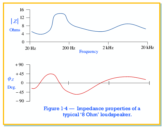
Figure 1·4 shows a typical example. In this case the loudspeaker has an impedance of around 12 Ohms at 150 Hz and 5 Ohms at 1 kHz. So over twice the current will be required to play the same output level at 1 kHz than is required at 150 Hz. The power amplifier has no way to “know in advance” what kind of loudspeaker you will use so simply adopts the convention of asserting a voltage level to indicate the required signal level at each frequency in the signal and supplying whatever current the loudspeaker then requires.
This kind of behaviour is quite common in electronic systems. It means that, in information terms, the signal pattern is determined by the way the voltage varies with time, and – ideally – the current required is then drawn. Although the above is based on a high-power example, a similar situation can arise when a sensor is able to generate a voltage in response to an input stimulus but can only supply a very limited current. In these situations we require either a current amplifier or a buffer. These devices are quite similar, in each case we are using some form of gain device and circuit to increase the signal current level. However a current amplifier always tries to multiply the current by a set amount. Hence is similar in action to a voltage amplifier which always tries to multiply the signal current by a set amount. The buffer differs from the current amplifier as it sets out to provide whatever current level is demanded from it in order to maintain the signal voltage it is told to assert. Hence it will have a higher current gain when connected to a more demanding load.
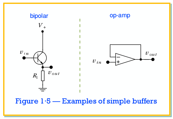
Figure 1·5 shows two simple examples of buffers. In each case the gain device (an NPN transistor or an op-amp in these examples) is used to lighten the current load on the initial signal source that supplies  . An alternative way to view the buffer is to see it as making the load impedance seem larger as it now only has to supply a small current to ensure that a given voltage is output.
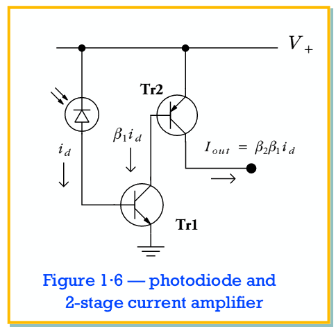
Figure 1·6 shows an example of a 2-stage current amplifier in a typical application. The photodiodes often used to detect light tend to work by absorbing photons and releasing free charge carriers. We can then apply a potential difference across the photodiode’s junction and ‘sweep out’ these charges to obtain a current proportional to the number of photons per second striking the photodiode. Since we would require around 1016 electrons per second to obtain an amp of current, and the efficiency of the a typical photodiode is much less than ‘one electron per photon’ this means the output current from such a photodector is often quite small. By using a current amplifier we can boost this output to a more convenient level. In the example, two bipolar transistors are used, one an NPN-type, the other PNP-type, with current gains of  and
and  . For typical small-signal transistors
  so a pair of stages like this can be expected to amplify the current by between × 250 and × 250,000 depending upon the transistors chosen. In fact, if we wish we can turn this into a voltage by applying the resulting output current to a resistor. The result would be to make the circuit behave as a high-gain voltage amplifier.